【www.zhangdahai.com--其他范文】
Qian ZOU, Quanjia ZHONG, Jiangyu MAO, Ruiqiang DING, Deyu LU, Jianping LI, and Xuan LI
1State Key Laboratory of Numerical Modeling for Atmospheric Sciences and Geophysical Fluid Dynamics (LASG),Institute of Atmospheric Physics, Chinese Academy of Sciences, Beijing 100029, China
2College of Earth Science, University of Chinese Academy of Sciences, Beijing 100049, China
3State Key Laboratory of Earth Surface Processes and Resource Ecology,Beijing Normal University, Beijing 100875, China
4Frontiers Science Center for Deep Ocean Multispheres and Earth System (FDOMES)/Key Laboratory of Physical Oceanography/Institute for Advanced Ocean Studies, Ocean University of China, Qingdao 266100, China
5Laboratory for Ocean Dynamics and Climate, Pilot Qingdao National Laboratory for Marine Science and Technology, Qingdao 266237, China
6Department of Atmospheric and Oceanic Sciences and Institute of Atmospheric Sciences,Fudan University, Shanghai 200438, China
ABSTRACT Based on a simple coupled Lorenz model, we investigate how to assess a suitable initial perturbation scheme for ensemble forecasting in a multiscale system involving slow dynamics and fast dynamics. Four initial perturbation approaches are used in the ensemble forecasting experiments: the random perturbation (RP), the bred vector (BV), the ensemble transform Kalman filter (ETKF), and the nonlinear local Lyapunov vector (NLLV) methods. Results show that,regardless of the method used, the ensemble averages behave indistinguishably from the control forecasts during the first few time steps. Due to different error growth in different time-scale systems, the ensemble averages perform better than the control forecast after very short lead times in a fast subsystem but after a relatively long period of time in a slow subsystem.Due to the coupled dynamic processes, the addition of perturbations to fast variables or to slow variables can contribute to an improvement in the forecasting skill for fast variables and slow variables. Regarding the initial perturbation approaches,the NLLVs show higher forecasting skill than the BVs or RPs overall. The NLLVs and ETKFs had nearly equivalent prediction skill, but NLLVs performed best by a narrow margin. In particular, when adding perturbations to slow variables,the independent perturbations (NLLVs and ETKFs) perform much better in ensemble prediction. These results are simply implied in a real coupled air—sea model. For the prediction of oceanic variables, using independent perturbations (NLLVs)and adding perturbations to oceanic variables are expected to result in better performance in the ensemble prediction.
Key words: ensemble prediction, nonlinear local Lyapunov vector (NLLV), ensemble transform Kalman filter (ETKF), coupled air—sea models
In recent years, air—sea coupled models which describe the interactions between the atmosphere and the ocean have been more extensively applied to simulate weather and climate phenomena (Bender et al., 2007; Zou et al., 2016; Larson and Kirtman, 2017; Mogensen et al., 2017). Air—sea coupling plays an important role in the simulation of weather and climate (Dong et al., 2017; Thompson et al., 2019). At the air—sea interface, material and energy are exchanged, along with many complex physical processes (Soloviev et al.,2014). Coupled models can describe these coupled feedback processes better than atmosphere-only models (Perlin et al.,2020). Hence, the simulation of weather and climate phenomena can be improved by using a coupled air—sea model (Fu and Wang, 2004; Wang et al., 2005; Ratnam et al., 2009;Dong et al., 2017).
However, the simulation of weather and climate phenomena using coupled air-sea models involves many uncertainties, including initial condition uncertainty (Lorenz, 1969,1982) and model uncertainty (Leutbecher and Palmer,2008). Ensemble prediction technology has evolved to reconcile these uncertainties (Leith, 1974; Ehrendorfer, 1997;Demeritt et al., 2007). It generates ensemble members by adding perturbations to the analysis state (Magnusson et al.,2008). The mean of the ensemble members can reduce the errors compared to a single forecast, and we can quantitatively estimate the probability density of a forecast state with a finite number of ensemble members (Froude et al., 2007;Leutbecher and Palmer, 2008; Feng et al., 2014).
Here, we mainly focus on ensemble prediction related to initial condition uncertainty. The key to constructing initial perturbations is to generate several initial states that can represent the initial uncertainty (Zhang and Krishnamurti, 1999).Many ensemble initial perturbation methods have been developed in succession, such as the Monte Carlo method (also called the random perturbation (RP) method (Leith, 1974)),the bred vector (BV) method (Toth and Kalnay, 1993, 1997),the singular vector (SV) method (Palmer et al., 1992), the ensemble transform Kalman filter (ETKF) method (Wang and Bishop, 2003), the ensemble transform with rescaling(ETR) method (Wei et al., 2006, 2008), the conditional nonlinear optimal perturbations (CNOPs) method (Mu and Jiang,2008) and the nonlinear local Lyapunov vector (NLLV)method (Feng et al., 2014, 2016, 2018; Ding et al., 2017).
Many studies have focused on ensemble prediction in atmosphere-only or ocean-only models, but it has not been explored extensively in air—sea coupled models. Ensemble prediction in coupled models seems more complex because of the different time scales of the ocean and the atmosphere(Liu et al., 2013). An initial error can also evolve on different time scales (Vannitsem, 2017). In addition, the feedback process between the coupled components makes the system highly sensitive to errors (Zhang et al., 2005). Hence, important issues in ensemble forecasting in coupled models which contain feedback processes at different time scales remain to be explored.
Therefore, this paper determines how to add appropriate ensemble initial perturbations to a multiscale system based on multiple initial perturbation methods. The system is called the coupled Lorenz model, characterized by a slow subsystem coupled with a fast subsystem (Boffetta et al.,1998; Ding and Li, 2012). The fast subsystem fluctuates approximately 10 times faster than the slow subsystem,which is close to the relative time scale between the atmosphere and the ocean (Wang et al., 2002). Therefore, we can assume the coupled Lorenz model to be a toy coupled airsea model.
The remainder of this paper is organized as follows. Section 2 introduces the coupled Lorenz model and the algorithms to obtain the BVs, ETKFs, and NLLVs. Section 3 presents the properties of RPs, BVs, ETKFs, and NLLVs in the multiscale system. Section 4 is a summary and discussion of our major findings.
2.1. Coupled Lorenz model
The model used in this study is the coupled Lorenz model. It couples two simple Lorenz63 models (Lorenz,1963) with different time scales. The first characterizes the slow dynamics, and the second characterizes the fast dynamics (Boffetta et al., 1998; Ding and Li, 2012). The governing equations include:

where the superscripts (s) and (f) denote the slow dynamics and fast dynamics, respectively. The physical parameters of the above equations are displayed in Table 1. The relative time scale c is a constant set to 10, indicating that the fast dynamics fluctuate approximately 10 times faster than the slow dynamics. It is close to the relative time scale between the ocean and the atmosphere, which is about 9 (Wang et al.,2002). The variations in the fast variables change much faster than the variations in the slow variables (Fig. 1). The uncoupled slow and fast Lorenz models (coupling coefficients εs=0,εf=0) exhibit chaotic dynamics, with their Lyapunov exponents greater than zero. In setting εs=10-2,εf=10, the maximal Lyapunov exponent in the coupled Lorenz model has a value of 11.5, close to the value from uncoupled fast Lorenz models (Boffetta et al.,1998), indicating that it is the error growth of the fast system that determines the maximal Lyapunov exponent in the coupled Lorenz model.
The associated attractor of the coupled system seems interesting from the physical parameters given in Table 1.The two-dimensional projections of the attractor are shown in Fig. 2. The slow dynamics appear to show a typical Lorenz model (Figs. 2a—c), whereas the fast dynamics seemmuch more chaotic (Figs. 2e—f). The attractor orbit for fast dynamics becomes denser and the rate of motion is accelerated (Figs. 2e—f).

Table 1. Physical parameters used in the coupled Lorenz model.
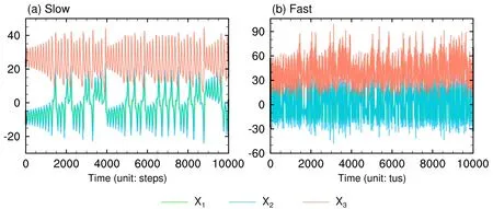
Fig. 1. Time evolution of variables for the coupled Lorenz model: (a) slow variables and (b) fast variables.

Fig. 2. Projections of the coupled Lorenz model on three two-dimensional planes: (a)—(c) for the slow variables and (d)—(f) for the fast variables.
2.2. Initial perturbation schemes
We use four methods to generate initial perturbations:RP, BV, ETKF, and NLLV. A brief description of the BV,NLLV, and ETKF methods follows.
2.2.1. Computation of the BVs
The BV method is based on the rationale that any initial random errors in the basic flow would evolve into the fastest growing directions (leading Lyapunov vectors) in phase space (Toth and Kalnay, 1993, 1997; Feng et al.,2014). The generation of BVs is described as follows. At first, a group of small initial random perturbations is added to the analysis state. After a period of integration (a breeding cycle), the differences between the control and perturbed forecasts are rescaled to the size of the initial perturbations. The rescaled difference fields will be added to the subsequent analysis. After repeating the process for several breeding cycles,the perturbation evolves into a fast-growing perturbation, generating the BVs. The following mathematical formulation is to describe the repeated process:

where the xcand xprepresent the control trajectory and perturbation trajectory, respectively. The term ε0p/‖p‖ represents the scaling, where ε0is a scaling factor and p is the difference between the control and perturbed forecasts.
2.2.2. Computation of the NLLVs
NLLVs are a nonlinear extension of the Lyapunov vectors (LVs) similar to BVs (Feng et al., 2014; Hou et al.,2018). Compared to BVs, different NLLVs are independent of one another and represent the fastest direction of error growth in different subspaces of the phase space. The generation of NLLVs is introduced below (Feng et al., 2014, 2016).As shown in Fig. 3, the leading NLLV (NLLV1), the fastestgrowing direction, can be obtained via a breeding process similar to creating a BV. The rest of the NLLVs can be obtained in each breeding cycle via a Gram—Schmidt reorthonormalization (GSR) process (Wolf et al., 1985; Feng et al., 2014). The evolved perturbations (grey dashed lines in Fig. 3) are orthogonalized with the leading NLLV(NLLVnare orthogonalized associated with NLLV1,NLLV2, NLLV3, …, NLLVn-1). The orthogonalized perturbations are then scaled back to the initial size and enter the next breeding process. After multiple breeding cycles, the NLLVs are produced. This paper"s breeding cycle for generating BVs and NLLVs lasted 0.05 time units (tus) and was repeated 20 times.

Fig. 3. Schematic diagram of the generation of NLLVs [adapted from Hou et al. (2018)]. The creation of NLLV1 is similar to the creation of BV. To acquire the NLLV2, a pair of RPs is initially added to the analysis state. The evolved perturbations (grey dashed line) are orthogonalized with the NLLV1 (blue dashed line) to produce the NLLV2 (green dashed line) using a Gram—Schmidt re-orthonormalization (GSR) procedure.Similarly, the vectors NLLVn are orthogonalized with NLLV1, NLLV2, NLLV3, …, NLLVn—1.
2.2.3. Computation of the ETKFs
The ETKF method, initially introduced by Bishop et al.(2001), was derived from ensemble-based data assimilation theory, which is associated with Kalman filtering (Wang and Bishop, 2003; Wei et al., 2006; Wu et al., 2009). Similar to the ensemble Kalman filter (EnKF), the ETKF method applies Kalman filtering to generate a sample analysis ensemble. However, the ETKF only uses the forecast error covariance matrix to estimate the analysis error covariance through a transformation matrix, not updating the mean state (Wang and Bishop, 2003; Zhou et al., 2019). The equation for the ETKF algorithm is as follows:

where Xaand Xfare denoted as the analysis perturbation and forecast perturbation matrix, respectively, and T is a transformation matrix. The detailed computation process follows Hunt et al. (2007). Localization is not used in this method. A multiplicative covariance inflation factor (set to 1.3) is applied. The observation was produced by adding a random perturbation (following standard Gaussian distribution) to the true state. Moreover, we use an ensemble size of 20, assimilated every 0.05 tus, and the performing time is over 1 tus.
Studies have shown that the ETKF can be used to generate ensemble perturbations and outperform most ensemble generation schemes in sampling the analysis uncertainties(Wei et al., 2006; Feng et al., 2016). One of the greatest attributes of ETKFs is that they are orthogonal in observational space (Wang and Bishop, 2003; Wei et al., 2006;Feng et al., 2016).
2.3. Experimental design
To clarify the performance of the evolution of the initial perturbations in a multiscale system as much as possible,we performed several ensemble forecasting experiments in the coupled Lorenz model based on RP, BV, ETKF, and NLLV methods. The model is integrated by a fourth-order Runge-Kutta method with a time step of 0.005 tus in all experiments. The procedure for the ensemble forecasting experiments is shown in Fig. 4. The first 10 000 steps involve a spin-up of the coupled Lorenz model. After spin-up, we use a 200-step ensemble Kalman filter (EnKF) data assimilation scheme (Evensen, 2003, 2004) to create the initial analysis state. The parameter set of the EnKF assimilation procedure is the same as for the ETKF scheme. The assimilation cycle is 0.05 tus, which is perfect to project to 6 hours window in real world. Hence, our 1 tus in this paper is 5 days in real world. During the assimilation process, the BV and NLLV perturbations are calculated based on the assimilated data as a basic flow. Then the ensemble perturbations created by the RP, BV, ETKF, and NLLV methods are added to the analysis state in pairs (both positive and negative perturbations are added). The ensemble perturbation vectors are scaled to 1 × 10—2. The integration from the analysis state is the control forecast, and the perturbed forecasts are ensemble members.By increasing the number of ensemble members, the prediction level of the ensemble forecast, which is driven by BVs,NLLVs, and ETKFs, showed improvement (not shown).Thus, the ensemble size is six pairs in this paper (with positive and negative perturbations superimposed in pairs). We ran 10 000 samples of the ensemble forecast (repeating the assimilation/breeding and forecasting processes). The initial value of each sample has one step interval. The initial states of 10 000 samples include a representative range of coupled model states.

Fig. 4. Illustration of the initialization and forecasting procedure. Numbers represent the integration steps,and 1 step = 0.005 tus.

Fig. 5. Panels (a)—(c) Evolution of control forecasts (light blue) against the true state (light red) as a function of lead time for (a) the whole system, (b)the fast subsystem, and (c) the slow subsystem (in the Euclidean norm). (d)Mean growth rate in the form of Lyapunov exponent (value × 100) of 10000 samples as a function of lead time from the coupled Lorenz model for the control run [the whole system (light purple), fast subsystem (light orange),and slow subsystem (light blue)].
2.4. Verification method

To evaluate the reliability of the ensemble predictions,a classical Brier score is applied to assess the relative skill of the BV compared with that of NLLV and ETKF. For any event ϕ, the Brier score (Brier, 1950) is computed as:where N is the number of samples, fidenotes the probability of the i-th sample for the prediction of event ϕ , and oidenotes the probability of the i-th sample actually occurring for event ϕ (which can take on values of only 0 or 1).
Before evaluating the quality of the ensemble predictions, the errors from the control forecast were investigated.We assumed that the model was perfect and the true state was a long model run for each sample. As shown in Fig. 5,a large difference exists between the control forecast and the true value. The evolution of the control and true value shows rapid fluctuating changes across the whole system(Fig. 5a). When separating the coupled Lorenz system into a fast and slow subsystem, similar characteristics are found in the fast subsystem compared to the whole system (Fig. 5b).However, the two time series in the slow subsystem are characterized by slow fluctuating changes that do not show a significant distinction until 4 tus into the simulation (Fig. 5c).Given the relatively large difference between the control forecast and the true state, we use the Lyapunov exponential form error growth rate to measure the variation of forecast error for the control run. We found that the initial error in analysis shows positive growth over time. The forecast error for a control run mainly comes from the fast subsystem. The variation in forecast error for the control run is different in the slow and fast subsystems, with the error growing much faster in the fast subsystem than in the slow subsystem(Fig. 5d). The equation for the Lyapunov exponential form error growth rate is as follows:

Fig. 6. Mean RMSE (solid lines) and ensemble spread (dashed lines) of 10 000 samples as a function of lead time for the control run (black), RP method (red), BV method (blue), ETKF method (purple), and NLLV method (green) after adding perturbations to all variables: (a) the whole system, (b) the fast subsystem, and (c) the slow subsystem.

where t0is the initial time, ‖△x(t)‖ denotes the error size in the Euclidean norm at time t.
Studies have proven that the ensemble forecast improves the quality of the control forecast (Toth and Kalnay, 1997; Ndione et al., 2020). Running an ensemble of forecasts by adding perturbations to initial conditions allows the ensemble mean to improve the prediction by filtering out unpredictable components, and the spread among the forecasts can provide a probability prediction (Toth and Kalnay,1993). To explore the appropriate ensemble initial perturbation configuration in a multiscale system, many ensemble forecast experiments are conducted in this part of the paper,with multiple perturbation methods (RP, BV, ETKF, and NLLV). The root-mean-square error (RMSE) for the ensemble mean and the ensemble spread are used to measure the forecast skill of the experiments. In a “perfect ensemble”,the ensemble spread will be close to the RMSE of the ensemble mean for all forecast times (Palmer et al., 2006; Magnusson et al., 2008; Buckingham et al., 2010). Considering the different error growth in the fast and slow subsystems, we shall discuss them separately. In Fig. 6, the mean RMSE(solid lines) and ensemble spread (dashed lines) are plotted for the control (black), RP (red), BV (blue), ETKF (purple),and NLLV (green) after adding the perturbations to all variables. The RMSE oscillates at short lead times. It is possible that the RMSE oscillation at short lead times is related to our temporal scale, which is similar to diurnal cycling. In the first 0.5 tus, the RMSE for the NLLV, ETKF, BV, and RP ensembles is similar to that of the control run. This is mainly because positive and negative perturbations superimposed on the control run cancel each other out at the initial time [errors grow linearly at the initial time (Ding and Li,2007)]. Soon thereafter, regardless of the perturbation method, the ensemble forecast can effectively reduce forecast errors from the control run in a general sense. In terms of the RMSE for the ensemble mean, the results from NLLVs are the lowest, followed by ETKFs, BVs, RPs, and the control forecast. Among these, NLLVs and ETKFs demonstrate nearly the same forecast ability. These two methods have obviously better predictive skill than the BVs in the two main periods: 0.5—2 tus and 4.5—8 tus (a smaller RMSE for the ensemble mean and bigger ensemble spread) (Fig. 6a).During the period of 0.5—2 tus, the better predictive skill of NLLVs and ETKFs over the whole system is reflected mainly in the reduction in forecast errors in the fast subsystem(Fig. 6b). This is reflected in the reduction in forecast errors in the slow subsystem during the 4.5—8 tus forecast period(Fig. 6c).
Next, we wonder whether adding perturbations to different variables of this system can achieve improvements from BVs to ETKF and NLLVs. Good ensemble perturbations should reflect the initial uncertainty of analysis (Toth and Kalnay, 1993). The ability to capture the initial uncertainties varies among different perturbation methods. Owing to the differing error growth for initial perturbations in fast and slow subsystems (Fig. 5d), the prediction skill for the various perturbation methods may differ when adding different timescale perturbations. To further clarify this issue, three error-addition schemes are used in this study: adding perturbations to both fast and slow variables, adding perturbations only to fast variables, and adding perturbations only to slow variables. Figure 7 shows that whether perturbations are added to fast variables or to slow variables, they contribute to an improvement in the forecasting skill for the fast variables due to the feedback process between the coupled components. When adding perturbations only to fast variables, the ensemble skills of all perturbation methods are improved when predicting fast variables after 0.4 tus (Fig. 7b). However, when adding perturbations solely to the slow variables,only the NLLVs and ETKFs can improve the prediction skill of fast variables during the 0.4—0.8 tus forecast period(Fig. 7c). In other words, only better independent perturbations superimposed on the slow subsystem can improve the forecasting skill of the fast subsystem.
The ensemble forecast of slow variables behaves differently than fast variables. The advantages of the ensemble forecast over the control forecast become apparent at 4 tus(Fig. 8). When adding perturbations only to fast variables,the forecasting skills of BVs, ETKFs, and NLLVs are equivalent (Fig. 8b). However, when adding perturbations only to slow variables, large differences are shown between the BVs, with NLLVs and ETKFs indicating that more independent perturbations lead to better prediction skill for the slow subsystem (Fig. 8c). Because of the feedback process between the coupled components, adding perturbations to both fast and slow variables improves the forecasting skill for the slow variables.
In general, the ensemble forecast performs differently in different time-scale systems. After a while, the ensemble forecast demonstrates better prediction skill than the control run. The advantages of the ensemble forecast become apparent after a very short period of time in a fast subsystem but after a relatively long period of time in a slow subsystem.The reason for this difference is associated with the different error growths of different time-scale systems. In fast dynamics, errors from the analysis state grow quickly, whereas they grow relatively slowly in slow dynamics. Besides,adding perturbations to both fast and slow variables contributes to an improvement in the forecasting skill for fast variables and slow variables, indicating that uncertainty in both fast and slow variables plays a role in their prediction.When adding perturbations to slow variables, independent perturbations (NLLVs and ETKFs) seem to perform much better than the other types (BVs or RPs) in predicting both fast and slow variables. This is likely because highly independent perturbations can better capture initial uncertainty information. Additionally, NLLVs appear to outperform ETKFs by a narrow margin (Figs. 6—8). To further confirm this, we conduct an independent sample t-test with the RMSEs of 10 000 samples for the ETKF and NLLV methods. The RMSE data are from the same experiments indicated in Fig. 6a. The mean RMSE from NLLV is less than that from ETKF (with a difference of —0.1429), exceeding the 90% confidence level (with a probability value of 0.0812; not shown). Therefore, of the two independent perturbations,the NLLV is better than the ETKF.
Other evidence also shows that the independent perturbations (NLLVs) demonstrate better forecasting skill than BVs. Figure 9 provides the distribution of the RMSEs and ensemble spreads from 10 000 samples for the NLLV and BV predictions. At the beginning of the ensemble forecast,the forecast errors for both NLLVs and BVs are concentrated mainly around the diagonal, indicating that the forecasting skill of NLLVs is roughly equal to that of BVs (Fig. 9a).The number of samples with a prediction error by NLLVs less than that by BVs increase over time, reaching 58% of total samples at 6 tus (Fig. 9b). The number of samples with an ensemble spread by NLLVs is greater than that for BVs at any time (Figs. 9d—f). We conclude that compared to BVs,NLLVs tend to have a smaller RMSE for the ensemble mean, and a bigger ensemble spread, indicating a better ensemble prediction performance.

Fig. 7. Mean RMSE (solid lines) and ensemble spread (dashed lines) of 10 000 samples in the fast subsystem as a function of lead time for the control run (black), random perturbation method (red), BV method (blue), ETKF method (purple), and NLLV method (green) after adding perturbations to different variables: (a) adding perturbations to both fast variables and slow variables,(b) adding perturbations only to fast variables, and (c) adding perturbations only to slow variables.

Fig. 8. Mean RMSE (solid lines) and ensemble spread (dashed lines) of 10 000 samples in the slow subsystem as a function of lead time for the control run (black), random perturbation method (red), BV method (blue), ETKF method (purple), and NLLV method(green) after adding perturbations to different variables: (a) adding perturbations to both fast variables and slow variables, (b)adding perturbations only to fast variables, and (c) adding perturbations only to slow variables.

Fig. 9. Panels (a)—(c) RMSE of 10 000 samples based on NLLV and BV methods at (a) 3 tus, (b) 6 tus, and (c) 9 tus in the slow subsystem. The upper right-hand corner indicates the ratio of samples where RMSE for the NLLV method is smaller than the RMSE for the BV method in (a)—(c). Panels (d)—(f) are the same as (a)—(c), but for an ensemble spread of 10 000 samples. The upper right-hand corner indicates the ratio of samples where the ensemble spread for the NLLV method is larger than for the BV method in (d)—(f). Panels (a)—(f) are based on the experiments which add perturbations to both fast and slow variables.
The Brier score (BS) is commonly used to evaluate the quality of probabilistic forecasts generated by ensembles(Stephenson et al., 2008). We choose the event ϕ1(foris the climatological mean to the distance of one standard deviation) (Fig. 10a) and event ϕ2(foris the climatological mean to the distance of one standard deviation)(Fig. 10b) to calculate the basic BS from an average of 10 000 samples. The smaller the BS value, the better the forecasting skill of the ensemble forecast. As shown in Fig. 10,the NLLVs are more skillful than BVs and RPs, and their performance is similar to ETKFs.
The other verification method used was the Talagrand diagram (also called rank histograms), which can characterize the reliability of an ensemble forecast (Talagrand et al.,1997; Candille and Talagrand, 2005). For a reliable ensemble forecasting system, the observation must fall with equal probability into any of the N+1 intervals divided by the N ensemble forecast values (Talagrand et al., 1997). Considering an ensemble forecasting system with N members, the predicted value,, can be defined as Pi,j, where i denotes the i-th sample, and j denotes the j-th ensemble member. For each sample, we count the number of members whose predicted values are smaller than the true values, represented as n, which can take on values of only 0-N. Then, we count the number of samples (for all samples of S, we run 10 000 samples of the ensemble forecast) under each n, defined by Sn. The ideal frequency of Snis S/(N+1), for which we expect the true value to have equal probability in the N+1 intervals. We then calculate the relative frequency Pn=Sn/[S/(N+1)]. The distribution of Pnis plotted in Fig. 11. It shows that the NLLV,ETKF, and BV ensembles are under-dispersive. But the results for NLLVs show a flatter histogram, indicating the greater reliability of the NLLV ensemble system. The stability of the NLLV and the ETKF ensemble systems is comparable. The results from BS and the Talagrand diagram are based on the ensemble experiment, which adds perturbations to both fast and slow variables. From this, we choose to analyze results fromand. Similar results can be obtained from other error-addition schemes and variables(not shown). These results prove that NLLVs and ETKFs perform better than BVs in the ensemble prediction.

Fig. 10. (a) Basic Brier score (BS) for the event ϕ1 (ϕ1: where is the climatological mean to the distance of one standard deviation) of ensemble forecasts based on NLLVs (green line), ETKFs (purple line), BVs (blue line), and RPs (red line) as a function of lead time. Panel (b) is the same as (a), but for event ϕ2 (ϕ2 : where is the climatological mean to the distance of one standard deviation).

Fig. 11. The histogram of the Talagrand distribution for different member intervals. The horizontal dashed lines denote the expected probability for the ensemble forecasts based on (a) BVs, (b) NLLVs, and (c) ETKFs at 2 tus. Panels (a)—(c) are based on the experiment which adds perturbations to both fast and slow variables and predicts the variable Panels (d)—(f) are the same as (a)—(c), but at 6 tus and predicted variable is .
Ensemble prediction remains a huge challenge in multiscale systems (Vannitsem and Duan, 2020). One important issue is how to generate appropriate perturbations for different time-scale variables. This issue has been addressed here by considering different time-scale initial perturbations in predicting different time-scale variables, noting that the selection of ensemble generation schemes is very important. The NLLV method has proven advantageous in ensemble forecasting (Feng et al., 2014, 2016; Hou et al., 2018). Therefore,we have explored how to add appropriate ensemble initial perturbations to a multiscale system based on multiple initial perturbation methods. The results are given below.
Compared to the control forecast, the ensemble forecast can effectively reduce forecasting errors in the coupled model. Due to different error growth in different time-scale systems, the advantages of an ensemble forecast become apparent after a very short period of time in a fast subsystem but after a relatively long period of time in a slow subsystem. We found that the dynamic processes among the slow and fast variables are coupled. This became evident when perturbations were added separately to a fast subsystem and a slow subsystem. Regardless of whether the perturbations were added to the fast or slow variables, there was an overall improvement in the forecasting skill for both the fast variables and slow variables.
In terms of initial perturbation methods, it is evident that independent perturbations (NLLVs and ETKFs) are superior to the other kinds (BVs or RPs). Both NLLVs and ETKFs had nearly equivalent prediction skill, with NLLVs having the greatest skill by a narrow margin. The ensemble forecasting system based on NLLVs or ETKFs is of higher quality than that based on BVs. In particular, when adding perturbations to slow variables, the highly independent perturbations (NLLVs and ETKFs) can capture initial uncertainty information quickly, giving them better prediction skill in the coupled system.
We may deduce that in a coupled ocean—atmosphere model, for the prediction of fast-scale variables (e.g., atmospheric variables), the ensemble forecast works on reducing the errors from the control forecast after a short time period.However, for slow-scale variables (e.g., oceanic variables),the ensemble forecast may effectively improve the medium and long-term forecasts. Consistent with air—sea coupling, adding perturbations to oceanic variables can improve the forecasting skill for atmospheric variables, and adding perturbations to atmospheric variables can also improve the forecasting skill for oceanic variables. When adding perturbations to oceanic variables, independent perturbations may perform better in the ensemble forecast of atmospheric and oceanic variables. These results may have important implications for the development of ensemble forecasts for coupled models in the future.
In general, NLLVs and ETKFs perform better than BVs and RPs in a coupled model. The computations of ETKFs require extensive computing resources. Fortunately,ETKF perturbations can be a byproduct of data assimilation.Compared to ETKFs, NLLVs are completely independent(orthogonal) and easy to calculate. Both NLLVs and ETKFs are expected to have a wide potential application in coupled models.
However, since we obtained these results through a toy model, further research is needed to expand these results to realistic air—sea coupled models. Our research team has attempted to apply NLLVs in the Weather Research and Forecasting (WRF) model. It is expected that NLLVs will exhibit a good performance in realistic air—sea coupled models. Besides, Vannitsem and Duan (2020) discovered that the fastest backward Lyapunov vectors are not optimal for initializing a multiscale ensemble forecasting system. Thus,choosing the appropriate NLLV modes in a multiscale ensemble forecasting system may be important. Both issues will be addressed in the near future.
Acknowledgements.This work was jointly supported by the National Natural Science Foundation of China (Grant Nos.42225501, 42105059).
本文来源:http://www.zhangdahai.com/shiyongfanwen/qitafanwen/2023/0903/648898.html